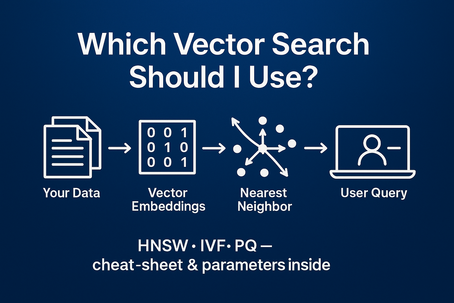
Modern AI applications from chatbots and recommendation systems to image search rely on searching high‑dimensional vectors. A well‑chosen index makes these searches fast and memory‑efficient, but there are many options. This guide answers a simple yet important question: which vector search index should you use?
We start with a gentle introduction to vector search and indexing, then explore the major index types: Hierarchical Navigable Small World (HNSW), Inverted File (IVF), Product Quantization (PQ) and the FAISS library that brings them together. For each index we explain what it is in plain language, why and when to use it, and dive into tuning parameters and trade‑offs. Finally, we provide a comparison table so you can quickly decide which index fits your use case.
What is indexing and vector search?
Imagine you have a million sentences, images or product descriptions represented as vectors, and you want to find the most similar items to a query vector. A naïve approach compares the query to every vector-accurate but slow. An index is a data structure built over your vectors that reduces the number of comparisons. When you search using the index, you sacrifice a tiny bit of recall for dramatic speedups.
Vector indexes fall into a few broad families:
-
Exact indexes: store vectors without approximation and perform brute‑force search. IndexFlatL2 in FAISS is a typical example and returns perfect results but scales poorly.
-
Cluster‑based indexes (IVF): partition vectors into clusters and search only the nearest clusters to the query.
-
Graph‑based indexes (HNSW): build a graph of vectors with long‑range and short‑range links and traverse it to find neighbors.
-
Compressed indexes (PQ): compress vectors into short codes so billions of vectors fit in memory.
In practice you’ll mix these techniques to balance recall, speed and memory. Let’s look at the major options and when to use each.
What does “recall” mean?
When we talk about approximate indexes, we often mention recall. Recall measures how many of the true nearest neighbors your search returns. A recall of 1.0 means your index found every nearest neighbor exactly. A recall of 0.9 means the index returned roughly 90 % of the true neighbors-often acceptable when search speed matters. Higher recall usually requires more computation or memory.
HNSW: Navigating a multi‑layer graph for high recall
What it is - simple terms
At its core, HNSW builds a multi‑layer graph. The top layer has a few long‑range “express” edges, while each lower layer contains more nodes and shorter edges. Searches start at the top, quickly traverse towards the query and then drop down to lower layers for fine‑grained comparisons. It’s like navigating from a highway to local roads.
The layered structure looks like this:
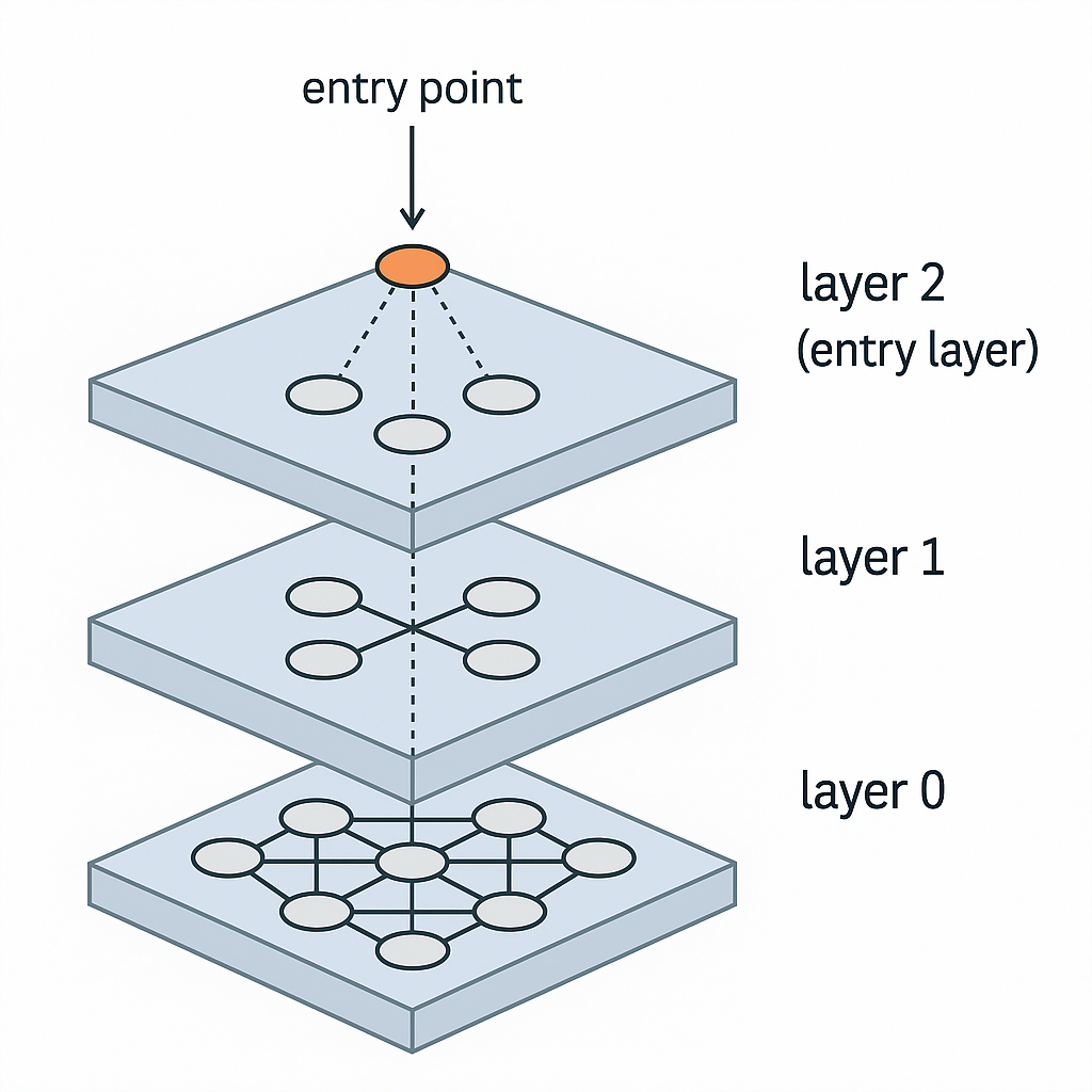 HNSW : Layered structure
HNSW : Layered structure
Why use HNSW
HNSW offers very high recall at low latency. Searches rarely miss relevant neighbors even with approximate traversal, and query times stay in the millisecond range. It allows incremental insertions, but deletions are generally handled via soft deletes and typically require periodic index rebuilding or graph maintenance to avoid fragmentation.
When to use HNSW
Choose HNSW when recall is paramount and you have enough memory. It’s ideal for semantic search on a few million documents or RAG (Retrieval Augmented Generation) pipelines where missing a key reference harms model outputs. Because HNSW stores raw vectors and graph edges, memory usage grows with data size, so it’s less suited to billions of vectors.
Tuning parameters, pros and cons
HNSW exposes three main parameters:
-
M - the maximum number of neighbors per node. Typical values range from 8 to 64; larger M increases recall but also memory usage and build time.
-
efConstruction - controls how thoroughly the graph is explored during construction. Recommended values often lie between 100 and 500; higher settings improve recall but slow indexing.
-
efSearch - the number of candidate neighbors examined during queries. For high‑recall applications, 100-200 or more is common; increasing this parameter raises recall at the cost of additional latency.
Pros:
-
High recall (>95%) and millisecond latency.
-
Supports incremental insertions. Deletions require soft‑marking of vectors and may necessitate rebuilding the graph to maintain performance
Cons:
-
Memory intensive. For 1 M 128‑dimensional vectors, the HNSW graph consumes ~128 MB and storing the raw vectors adds another ~512 MB.
-
Longer build times compared with cluster‑based methods.
IVF: Clustering vectors for efficient search
What it is - simple terms
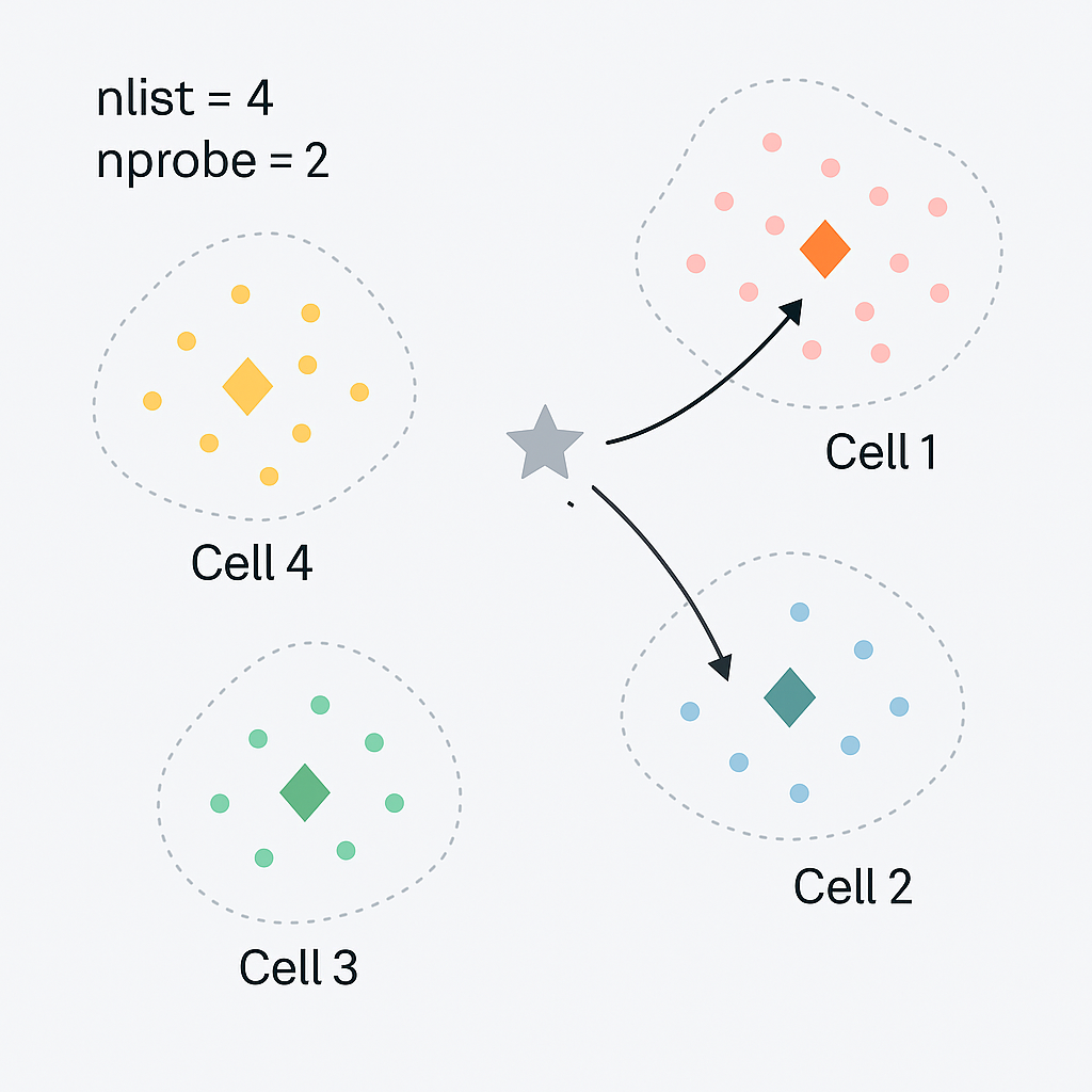
The Inverted File (IVF) index uses K‑means clustering to divide vectors into nlist clusters. At query time it only searches the top nprobe clusters closest to the query, reducing the number of vector comparisons. Think of it as grouping books by topic and only browsing relevant shelves.
This simplified diagram shows three clusters (cells). A query near the boundary benefits from increasing nprobe to search neighboring cells.
 IVF : Clustering and search
IVF : Clustering and search
Why use IVF
IVF delivers a good balance of speed, recall and memory. It’s faster than brute force because it searches fewer vectors, and memory overhead is modest since you only store centroids and an inverted list mapping vectors to clusters. It’s easy to implement and tune.
When to use IVF
IVF is suitable for large but not enormous datasets (millions to tens of millions) where you need decent recall and real‑time latency-such as product recommendations, deduplication or general vector search. For extremely large collections or tight memory budgets, combine IVF with PQ.
Tuning parameters, pros and cons
-
nlist - number of clusters. A good starting point is nlist ≈ 4 × √N (where N is the number of vectors); more clusters increase build time but reduce vectors per cluster and speed up search.
-
nprobe - number of clusters to search. Higher values improve recall but slow queries.
Pros:
-
Balanced memory and latency; memory around 520 MB for 1 M vectors.
-
Simpler to build and update compared with HNSW.
Cons:
-
Recall depends heavily on nprobe. Too small a value can miss neighbors near cluster boundaries.
-
Training is required and full re‑training may be needed when data distribution changes.
PQ: Compressing vectors for billion‑scale search
What it is - simple terms
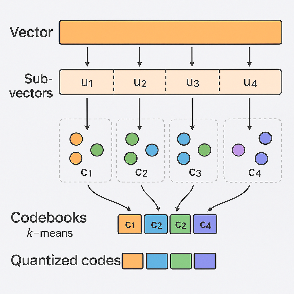
Product Quantization (PQ) compresses vectors into short codes. Each vector is split into m sub‑vectors; for each sub‑vector we learn a small codebook of centroids (e.g., 256 centroids). Instead of storing raw floats, we store the index of the closest centroid for each sub‑vector. This reduces storage dramatically.
The compression process is illustrated below:
 Product Quantization : Vector Compression
Product Quantization : Vector Compression
Why use PQ
PQ enables you to hold hundreds of millions or even billions of vectors in memory. On a 100 M‑vector dataset with 768‑dimensional embeddings, PQ compressed the index from 300 GB to 50 GB. It’s essential when memory is constrained but you need high throughput.
When to use PQ
Use PQ (often paired with IVF as IVF‑PQ) when your dataset is extremely large and storing raw vectors is impractical. This is common for large recommendation systems, deduplication of web‑scale corpora and some RAG retrieval tasks where moderate recall is acceptable.
Tuning parameters, pros and cons
-
m (number of sub‑vectors) - more sub‑vectors yield higher fidelity but longer codes. Choose m so each sub‑vector is 8-16 dimensions.
-
nbits - bits per sub‑vector (e.g., 8 bits for 256 centroids). More bits improve accuracy but increase memory.
-
refine_factor - number of candidates to re‑rank using original vectors.
Pros:
-
Massive memory savings; for a typical 128‑dimensional vector, PQ compresses the 512‑byte float32 representation down to about 8 bytes (≈ 98 % reduction). On very large, high‑dimensional datasets, reductions of around 6× have been reported (e.g., compressing a 100 M‑vector, 768‑dimensional index from 300 GB to about 50 GB)
-
Enables scaling to billions of vectors with modest hardware.
Cons:
-
Lower recall than raw-vector indexes; re‑ranking is usually necessary to achieve high accuracy.
-
More complex to tune (choice of m, nbits, cluster parameters and refine factor).
FAISS: A versatile toolkit
What it is - simple terms
FAISS (Facebook AI Similarity Search) is a library that implements a variety of vector indexes-including HNSW, IVF, PQ and combinations like IVF‑PQ. It offers both CPU and GPU implementations and provides utilities to tune index parameters.
How FAISS supports these index types
-
IndexFlatL2 and IndexFlatIP: exact indexes for L2 and inner product metrics.
-
IndexIVFFlat: cluster‑based IVF index. You supply a quantizer (IndexFlatL2), specify nlist, train on your data and set nprobe before searching.
-
IndexHNSWFlat: graph‑based HNSW index. You choose M, set efConstruction and efSearch, add vectors and query.
-
IndexIVFPQ: IVF with PQ compression. Create with nlist, number of sub‑quantizers (m) and bits per sub‑vector (nbits), train and add data.
FAISS also includes utilities like ParameterSpace and index_factory to automate parameter tuning and mixing index types. If you have GPUs, FAISS can offload distance computations to achieve even higher throughput.
Further tech details
 FAISS : Indexing and Search
FAISS : Indexing and Search
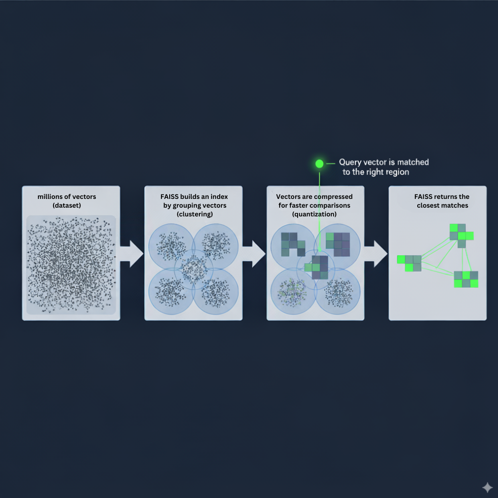
In FAISS, you’ll typically:
-
Generate or load your dataset: a NumPy array of shape (n_vectors, d) of type float32.
-
Build the index: choose an index class and pass dimension d and other parameters. Some indexes require training (e.g., IVF and PQ) while others (HNSW) do not.
-
Add vectors: call index.add(xb) to add your dataset.
-
Tune search parameters: set nprobe (IVF), efSearch (HNSW) or refine factors (PQ) to balance recall and speed.
-
Search: call index.search(query_vectors, k) to retrieve the k nearest neighbors and distances.
Choosing the right index: cheat sheet
The values below are approximate and depend on your data distribution, vector dimensionality, hardware and chosen hyper‑parameters. Use them as rough guidance and always benchmark on your own dataset.
To help you decide quickly, here’s a comparison of the index types on a 1 M‑vector, 128‑dimensional dataset. Ranges show how tuning parameters affect performance.
Index
Memory usage (approx.)
Query latency
Recall range
When to use
HNSW
≈600-1600 MB
≈0.6-2.1 ms
≈0.9-0.99(higher with larger efSearch)
High‑recall semantic search and RAG on millions of vectors; memory not constrained
IVF
≈520 MB
≈1-9 ms
≈0.7-0.95 (depends on nprobe)
Product search, deduplication, large datasets needing balanced speed and memory
IVF‑PQ
≈100-200 MB (depends on code length)
≈2-10 ms
≈0.6-0.9 before refinement; >0.9 with re‑ranking
Billion‑scale datasets where memory is tight; high throughput recommendations
HNSW‑PQ
≈136 MB for 1 M vectors
≈1-3 ms
≈0.8-0.95
Large semantic search or RAG where memory is limited but high recall is desired
FAISS Flat
≥500 MB
≈18 ms
1.0 (exact)
Small datasets or offline batch jobs where exact results matter more than latency
TL;DR recommendations
-
If recall is critical and memory is available: choose HNSW. Start with M in the 16-64 range and adjust efSearch (often 100-200 or higher) to achieve your recall
-
If your dataset is large and you need balanced performance: start with IVF using nlist ≈ 4×√N and tune nprobe for recall. Combine with PQ for billion‑scale datasets.
-
If you have a huge dataset and memory is tight: use IVF‑PQ or HNSW‑PQ. Re‑rank the top results with the original vectors to recover accuracy.
-
If you just need something simple for a few thousand vectors: the exact IndexFlatL2 is fine.
These recommendations are broad guidelines; the optimal index type and parameter settings depend heavily on your data distribution, dimensionality, hardware and recall/latency requirements, so always benchmark and tune on your own dataset.
Conclusion:
Vector search is a trade‑off between accuracy, speed and memory. The right index depends on your constraints and application. By understanding how HNSW, IVF and PQ work and tuning their parameters, you can build a search pipeline that performs well on your data.
References:
[1] [8] [11] Nearest Neighbor Indexes for Similarity Search | Pinecone
https://www.pinecone.io/learn/series/faiss/vector-indexes/
[2] Hierarchical Navigable Small Worlds (HNSW) | Pinecone
https://www.pinecone.io/learn/series/faiss/hnsw/
[3] [12] Product Quantization in Postgres | Lantern Blog
[4] [6] Vector Database Basics: HNSW | TigerData
https://www.tigerdata.com/blog/vector-database-basics-hnsw
[5] Index Explained | Milvus Documentation
https://milvus.io/docs/index-explained.md
[7] The Hierarchial Navigable Small Worlds (HNSW) Algorithm | Lantern Blog
[9] How can the parameters of an IVF index (like the number of clusters nlist and the number of probes nprobe) be tuned to achieve a target recall at the fastest possible query speed? - Zilliz Vector Database
[10] How do I tune hyperparameters for vector search?
https://milvus.io/ai-quick-reference/how-do-i-tune-hyperparameters-for-vector-search
[13] Mastering Faiss Vector Database: A Beginner's Handbook
https://www.pingcap.com/article/mastering-faiss-vector-database-a-beginners-handbook/
[14] Deep Dive into Faiss IndexIVFPQ for vector search | siddharth's space
https://sidshome.wordpress.com/2023/12/30/deep-dive-into-faiss-indexivfpq-for-vector-search/
[15] FAISS: The Key to Scalable, High-Dimensional AI Search